This time, we will introduce the Digital Pulse Processor (DPP), which digitizes waveforms for analysis.

There are various types of waveforms, ranging from logic waveforms like TTL to pulse waveforms from radiation detectors. The pulse widths also vary, from several milliseconds to several microseconds, and even down to nanoseconds.

Digital Pulse Processors are particularly well-suited for analyzing high-speed pulse waveforms, such as those from radiation detectors—especially scintillation detectors—ranging from several hundred nanoseconds to a few nanoseconds.

In this report, we will use the APV8104-14, one of our many Digital Pulse Processor products, equipped with a 1Gsps, 14-bit ADC. We will briefly explain the process from signal input to digital pulse processing, and then focus on explaining the QDC (Charge Digital Converter).

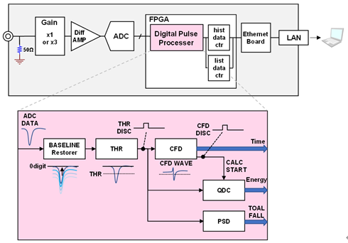
The input waveform is received with a 50Ω input impedance. The amplitude of the waveform is adjusted using gain from a high-speed amplifier circuit or an attenuator, and then digitized by the ADC.

The digitized waveform is digitally processed within the FPGA, allowing extraction of energy information (QDC), timing information (TDC), and pulse shape discrimination information (PSD). This information is useful for various physical measurement experiments. Let’s take a closer look at the signal processing section within the FPGA.

The internal signal processing is divided into several modules:
the Threshold Discriminator module, which serves as the starting point of signal processing; the CFD module for obtaining high-precision timing information; the QDC module for energy information; and the PSD module for pulse shape discrimination.

Each module performs calculations using FPGA’s characteristic parallel processing and pipeline processing. Although some latency occurs due to pipeline processing, the system can handle high-rate signal inputs with minimal dead time.

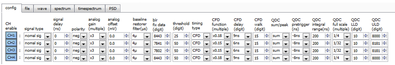
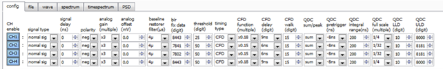
The parameters that can be set for each module are as follows.

The included application allows for fine-grained parameter configuration, providing a high degree of flexibility in adjustment.

Unlike conventional analog methods, fine-tuning can be easily performed on a computer, which is one of the major advantages of a digital system.

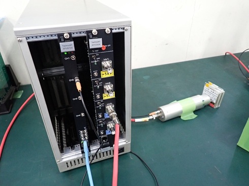
In practice, we conducted measurements using Techno AP’s 1-inch LaBr₃(Ce) detector model XL100 in combination with the digital pulse processor APV8104.

As radiation sources, a Cs-137 and Co-60 coincidence source was used. For the high-voltage power supply, we employed Techno AP’s APV3304.

The 1-inch LaBr₃ detector on the right integrates a scintillator, a photomultiplier tube (PMT), and a divider circuit into a single unit. To take full advantage of the fast decay characteristic of the LaBr₃ scintillator, the anode output of the PMT is provided directly.

This direct anode signal is connected straight to the digital pulse processor APV8104, resulting in a very simple measurement setup.
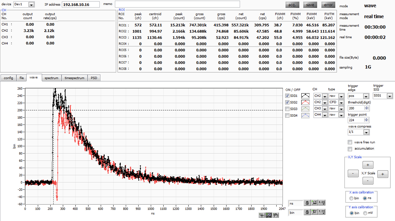
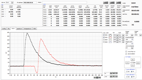
The digital pulse processor offers three primary measurement modes: wave mode, hist mode, and list mode.

Typically, the waveform is first observed in wave mode, followed by energy spectrum acquisition in hist mode. In wave mode, both the raw digitized waveform from the ADC and the CFD-shaped waveform generated by the CFD module can be observed. This serves as a convenient oscilloscope-like function within the software.

The figure below shows an example of the output display in wave mode as seen in the application.

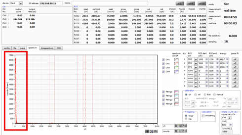
Next, we acquire the energy spectrum using hist mode.

The PMT converts incident light into electrons and amplifies them through multiple stages, with the signal ultimately reaching the anode. The anode signal is received by the digital pulse processor, which has an input impedance of 50 Ω. As electrons pass through, a potential difference is generated across this impedance.

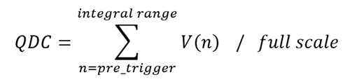
The energy information is obtained by simply summing this potential difference over time. The duration over which the summation takes place corresponds to the parameter Integral range (integration time).

The concept of the Integral range is illustrated as follows.

Integration begins at the Threshold point.

It is important to set the integration time with sufficient margin to fully cover the entire waveform.
Based on observations in wave mode, we determined that at least 100 ns was necessary, so in this case, we set it slightly longer at 144 ns.

However, by the time the threshold is triggered, the waveform has already started rising. Ideally, integration should begin earlier—before the threshold point.
This earlier start time is defined by the pre-trigger setting.

The concept of pre-trigger is illustrated as follows.

In the case of a LaBr₃ detector, the signal rises very quickly, so a pre-trigger setting of −8 ns is sufficient.
The integrated value obtained is ultimately multiplied by the full scale factor and reflected in the energy spectrum. The sequence of calculations leading to the final processed energy value is as follows:

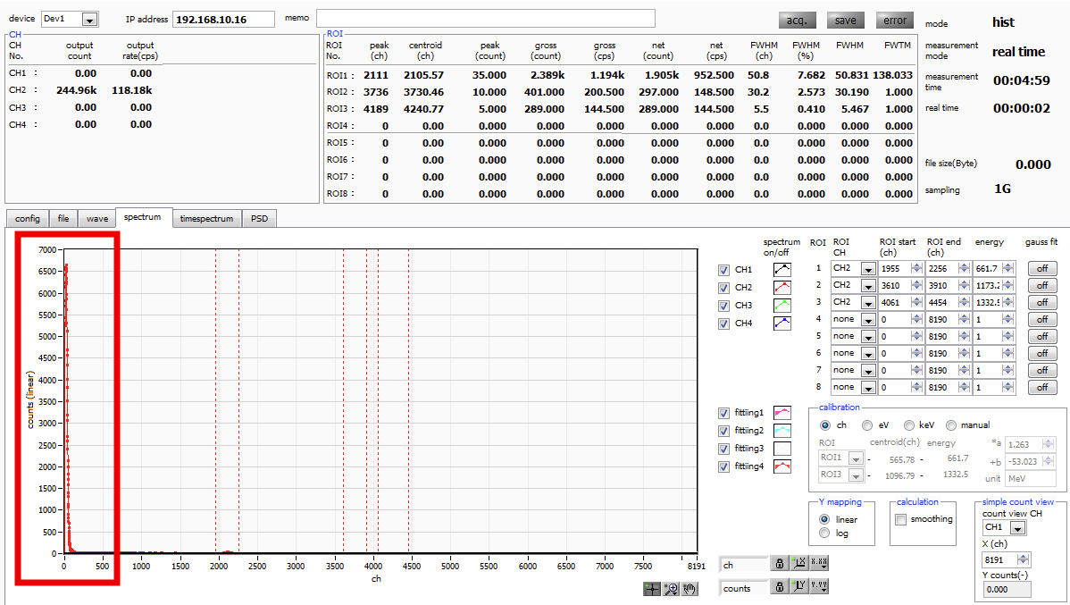
When measuring the energy spectrum, a prominent peak appeared on the low-energy side. This may indicate that the threshold is being triggered by noise.

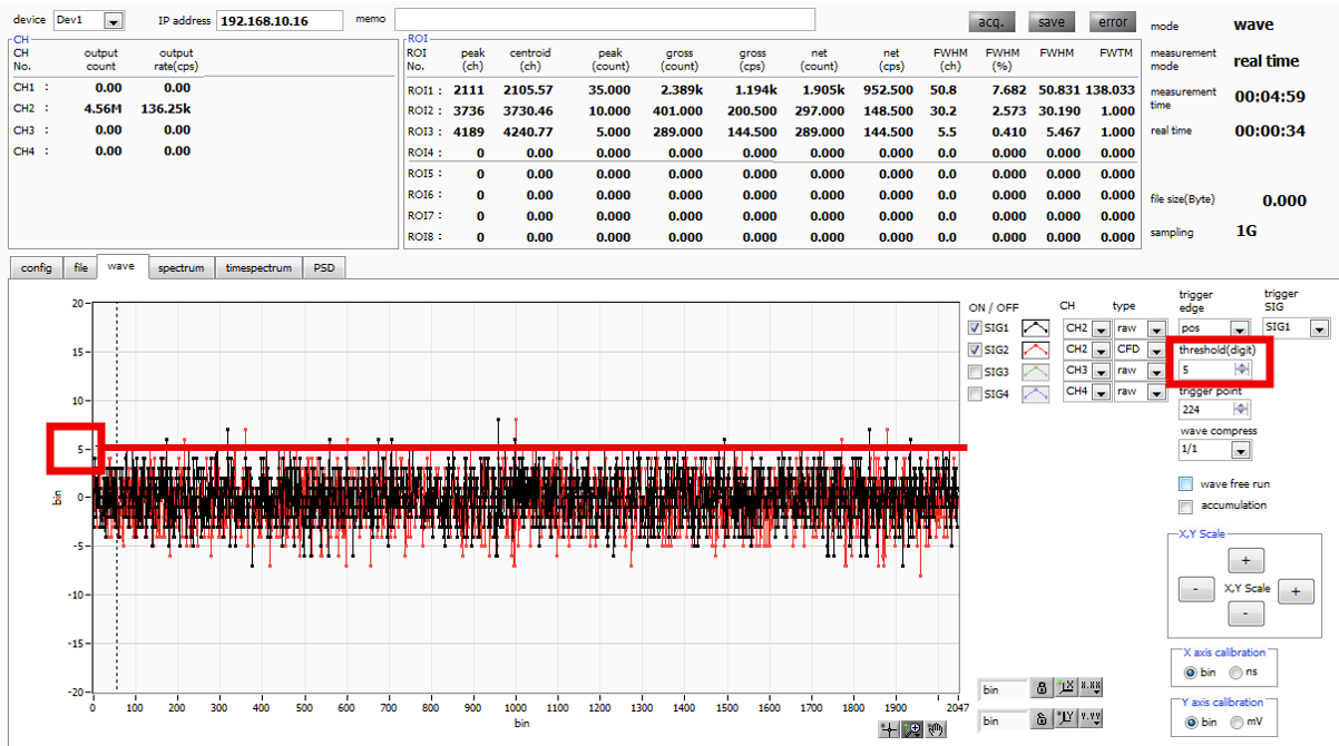
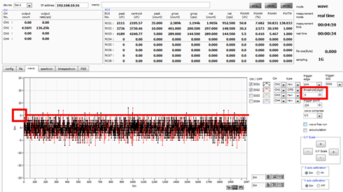
We will check the waveform again in wave mode.

The current threshold was set to 5 digits, so we input the same value, 5 digits, in the threshold setting section of the wave tab and perform the measurement.
As expected, we observed that many noise signals were indeed being triggered.

The upper edge of the noise appears to be around 8 digits.
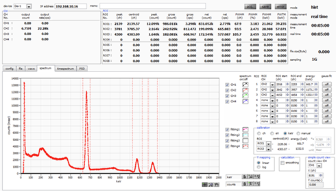
We will set the threshold value slightly above this level to ensure noise is excluded. In this setup, the threshold was set to 15 digits. We will now reacquire the energy spectrum.

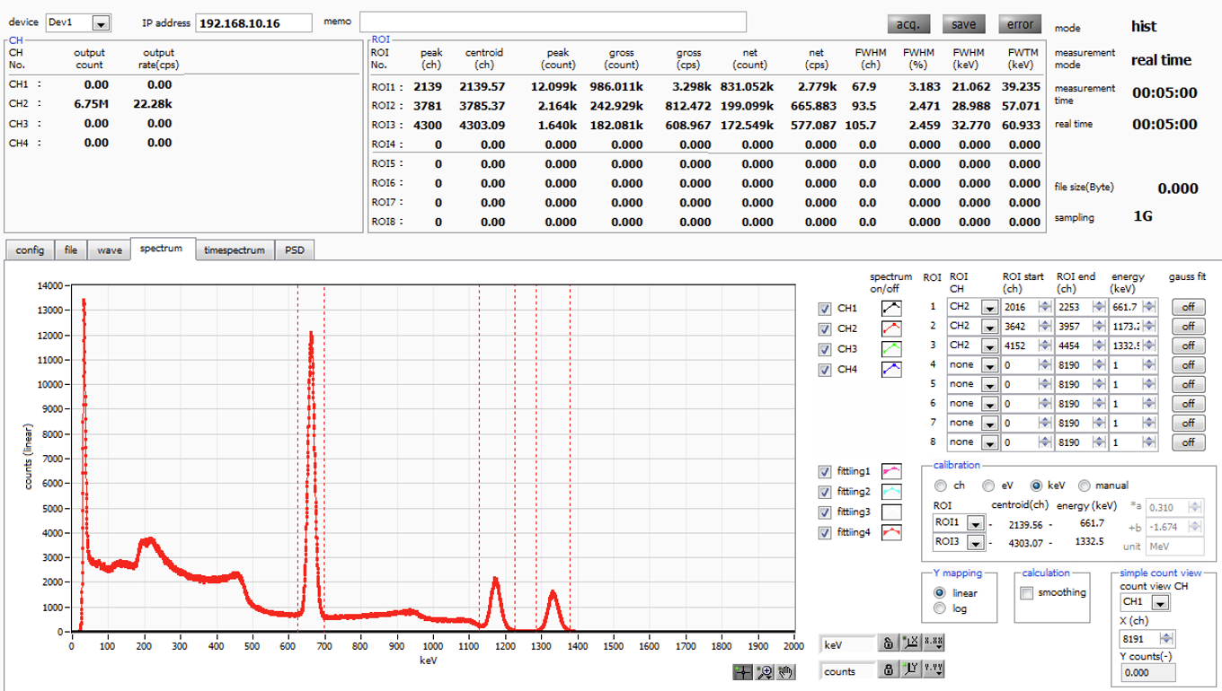
This time, the noise peak on the low-energy side disappeared, and a clean energy spectrum was obtained.

For the 662 keV peak from Cs-137, the measured energy resolution was 3.18%. Although the measurement setup is quite simple, it delivers excellent energy resolution.

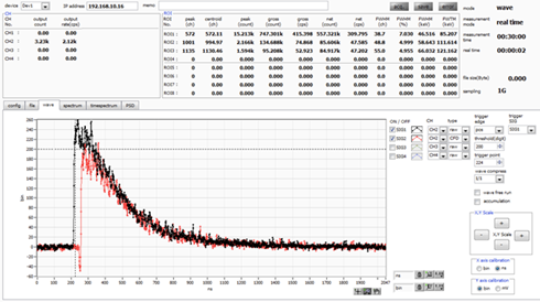
Since we have the opportunity, we also measured the energy spectrum using Techno AP’s 1-inch NaI detector. This detector is also a custom model with direct anode output. First, we check the waveform in wave mode.

The waveform width was approximately 800 ns until it fully decayed.

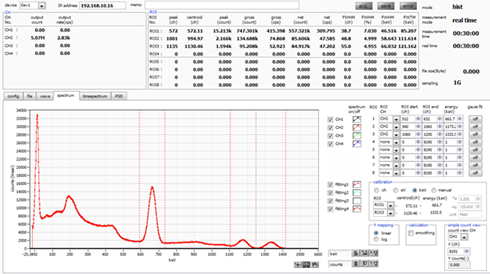
As expected, it is relatively long, so we set the Integral range to 1000 ns. We will now proceed to acquire the energy spectrum.

The energy resolution for the 662 keV peak from Cs-137 was 7.03%. This result can be considered fairly reasonable.

As demonstrated, the digital pulse processor is a convenient module that allows setup and measurement to be completed in just a matter of tens of minutes. We highly encourage you to give it a try.

In the next report, we will cover “Acquiring Time Difference Spectra (TDC) Using the Digital Pulse Processor.”

With that, our entire team remains committed to developing even better products. We sincerely appreciate your continued support and encouragement.